Finding the Median and an Application to Sorting

In the previous few entries we’ve been discussing quick_sort and analyzing the run-time complexity of recursive algorithms. We’re going to apply what we’ve learned so far to finding the median of an array in \(O(n)\) time. Then we’re going to see how that can be added to quick_sort to guarantee that it finishes in \(O(n\log_2(n))\) time.

The program we’re going to provide and discuss in this entry is more general than one that just finds the median. Given an array of integers of length \(N\) and a \(k\), such that \( 0 \leq k < N\), then our program will move all of the \(k\) smallest elements of the array to the first \(k\) positions. For example, if our original array is

\[ [ 97_{0}, 54_{1}, 11_{2}, 60_{3}, 66_{4}, 27_{5}, 20_{6}, 78_{7}, 63_{8}, 67_{9} ] \]

(where the subscript represents the index in the array), so that \(N = 10\), and we let \(k = 3\), then the output might be something like

\[ [ 27_{0}, 11_{1}, 20_{2}, 54_{k = 3}, 78_{4}, 60_{5}, 63_{6}, 97_{7}, 66_{8}, 67_{9} ]\]

Notice that our indexing of the elements of the array starts at \(0\), so the \(4^{th}\) position has index \(3\). The resulting element with index \(3\) is the \(4^{th}\) smallest element of the array. What’s more, everything to the left of it is smaller than or equal to it, and everything to the right of it is greater than or equal to it. In our case all of the inequalities are strict, because each element is unique.

Using this program, you can determine the median of an array. If the array has an odd number of elements, say, \(N = 2n + 1\), then the median is found by setting \(k = n\). The program doesn’t return that value, but you would then know that the element with index \(n\) is the median. On the other hand, if the array has an even number of elements, so \(N = 2n\), then we can determine the median by setting \(k = n\), once again, and then finding the maximum element to the left of position \(n\). What’s significant about this is that we can accomplish all of this without having to bother to sort the entire array. As mentioned above, our algorithm’s time complexity, \(T(n)\) is an element of \(O(n)\), which we will prove later in this entry. That’s much better than the upper bound we’ve proven for quick_sort.

To be fair, so far we haven’t proven that the worst case run-time for quick_sort is actually \(O(n^2)\). It is, and we’ll show that later. For now, let’s dig in to this new algorithm which separates an array into lesser and greater elements. We’ve implemented it in C++. Here’s the first function involved, it’s quite similar to what quick_sort does.

pivot()

 1
 2
 3
 4
 5
 6
 7
 8
 9
10
11
12
13
14
15
16
17
18
19
20
21
22
23
24
25
26
27
28
29
30
31
32

/*
  Let b = pivot(input, length). Then a < b < c
  implies that input[a] < input[b] <= input[c].
  
  input[b] is where input[0] is moved to at the
  end of execution.
*/

int64_t pivot(int64_t* input, int64_t length)
{
  int64_t i, j, tmp;
  i = 0;
  j = length - 1;

  while (i < j)
  {
    tmp = input[i+1];
    if(input[i+1] < input[i])
    {
      input[i+1] = input[i];
      input[i] = tmp;
      i++;
    }
    else
    {
      input[i+1] = input[j];
      input[j] = tmp;
      j--;
    }
  }// i == j
  return i;
}

quick_sort is nothing more than repeatedly calling pivot() on successively smaller sub arrays of the initial input array. pivot()’s running time is \(O(n)\), where \(n\) is the length of the input array. Notice that this function takes an array of int64_ts as its input, instead of a vector, which we used in our implementation of quick_sort. We chose this because it’s slightly simpler and doesn’t take away from the point of the algorithm.

The next function we’ll discuss is bubble_sort. It’s fine to use to sort short arrays. What’s nice about it is that it only involves two for loop and it avoids using any recursion.

bubble_sort()

 1
 2
 3
 4
 5
 6
 7
 8
 9
10
11
12
13
14
15
16
17
18
19
20

/*
  Runs in O(n^2) time, only use on small arrays
*/
void bubble_sort(int64_t* input, int64_t length)
{
  int64_t i, j, tmp;

  for(i = 0; i < length; i++)
  {
    for(j = i+1; j < length; j++)
    {
      if(input[j] < input[i])
      {
        tmp = input[i];
        input[i] = input[j];
        input[j] = tmp;
      }
    }// the j loop makes array[i] at least as small as everything to the right
  }
}

You can see we’ve mentioned in the comments above the implementation of the function that it runs in \(O(n^2)\) time, where \(n\) is the length of the input array. The reason why including this function in our algorithm doesn’t mean that the running time of kth_smallest() is an element of \(O(n^2)\) is that it is only ever runs on arrays of length CHUNK_SIZE or smaller. Typically CHUNK_SIZE is equal to 5. Finally, we introduce the function which combines the above two, and ultimately separates the array.

kth_smallest()

 1
 2
 3
 4
 5
 6
 7
 8
 9
10
11
12
13
14
15
16
17
18
19
20
21
22
23
24
25
26
27
28
29
30
31
32
33
34
35
36
37
38
39
40
41
42
43
44
45
46
47
48
49
50
51
52
53
54
55
56
57
58
59
60
61
62
63
64
65
66
67
68
69
70
71
72
73
74
75
76
77
78

// CHUNK_SIZE is usually 5 //
void kth_smallest(int64_t* input, int64_t k, int64_t length)
{
  if (length <= CHUNK_SIZE)
  {
    bubble_sort(input, length);
    return;
  }

  int64_t i, j, m_index, tmp, tmp_length;

  for (i = 0, j = 0; i < length; i+= CHUNK_SIZE, j++)
  {
    tmp_length = i + CHUNK_SIZE < length ? CHUNK_SIZE : length - i;
    bubble_sort(&input[i], tmp_length);

    // the index of the median of the small subarray
    m_index = i + tmp_length / 2;

    tmp = input[m_index];
    input[m_index] = input[j];
    input[j] = tmp;
  }
  /*
  This array replaces the front portion of input[] with the
  medians of the small subarrays.

  j is now equal to the length of the front portion of input[]
  */

  m_index = j / 2;
  kth_smallest(input, m_index, j);

  /* 
  m_index is the index of the median of the medians,
  which is where the name of the algorithm originates.
  */

  tmp = input[m_index];
  input[m_index] = input[0];
  input[0] =  tmp;

  m_index = pivot(input, length);

  /*
  We moved the median of the medians into input[0], which
  means that pivot will move everything < the median of medians
  to the left of m_index, and everything >= to the right.

  Note that the median of the medians is guaranteed to be greater than
  or equal to (j/2)*3 elements of input[].
  */

  // m_index is exactly where we want it. Nothing more to do.
  if (m_index == k)
  {
    return;
  }

  /*
  k is to the right of m_index, so we have to search among
  the right part of the array.

  Notice that we have to subtract m_index + 1 from the value
  of k and the length, because we're on the right side of
  m_index.
  */
  if (m_index < k)
  {
    kth_smallest(&input[m_index + 1], (k - (m_index + 1)), length - (m_index + 1));
  }

  /*
  k is to the left of m_index, so we have to search among
  the left part of the array
  */
  kth_smallest(input, k, m_index);
}

We’re going to show that \(T(n)\), the number of steps kth_smallest() takes to finish on an input array of length \(n\) is equal to \[ T(n) = c\left\lceil{ 0.2n }\right\rceil + T(\left\lceil {0.2n} \right\rceil) + T( \left\lceil { 0.7n } \right\rceil ) \tag{1}\label{1}\]

We’re going to assume that CHUNK_SIZE \(= 5\) in our analysis.

The leftmost term \(c\left\lceil{ 0.2n }\right\rceil\) comes from the bubble sorts. Each one takes \(c\) time. Easy enough. Then the next term comes from recursively calling kth_smallest() on the sub array of medians. This sub array has length \(\left\lceil {0.2n} \right\rceil\). Easy enough. Now let’s handle the rightmost term.

This comes from the two possible recursive calls to kth_smallest() at the end of the function. We want to show that we’ve eliminated at least \(\left\lfloor{0.3n}\right\rfloor\) elements from the input to the next function call. We’ll ignore the case where m_index == k, because then there’s no more work left to do. Case 1 is where m_index < k, so k is to the right of m_index.

Let’s stop for a bit to consider what m_index is. It is the index of the “median of the medians” (as mentioned in the comments to the code above). Let \(n = 5q + r\), then m_index is at least as large as \(3\left\lfloor {\frac{q}{2}} \right\rfloor\). This is because there are at least \(\left\lfloor {\frac{q}{2}} \right\rfloor\) “medians” (of the groups of 5) less than or equal to the element at m_index. Each one of those medians was at least as large as the two smaller elements in its group of 5. Therefore, each of those \(\left\lfloor {\frac{q}{2}} \right\rfloor\) groups of 5 had at least 3 elements less than or equal to the element at index m_index. Thus the element at m_index is greater than or equal to \(3\left\lfloor {\frac{q}{2}} \right\rfloor\) elements of the input array. We can rewrite this as \(\left\lfloor{\frac{n-r}{10}}\right\rfloor\), where \(r < 5\). This isn’t quite what we wanted, so maybe it’s better to say that we’ve eliminated at least \(\left\lfloor{0.29n}\right\rfloor\) of the original array for large enough \(n\). This is still good enough.

Case 2 where m_index > k is similar.

Now that we’ve (basically) shown that equation (1) holds, notice that \(\left\lceil {0.2n}\right\rceil \leq 0.2n + 1 \), and similarly, \(\left\lceil{ 0.7n }\right\rceil \leq 0.7n + 1 \). This means that their sum is less than or equal to \( 0.9n + 2 \). We will ultimately show that \(T\) is linear, but we don’t even need all of that for this next step. All we need to do is assume that \(T\) is convex (sometimes called “concave up” in calculus) and \(T(0) = 0\) to conclude that

\[T(m_1) + T(m_2) \leq T(m_1 + m_2) \]

We prove that with the following lemma.

Lemma (linear inequality)

Proof

The real power of the proof comes from the definition of convexity. \(S\) is convex if and only if

$$ \begin{align} &S( (1 - \lambda)x_1 + \lambda x_2 ) \\ &\leq (1 - \lambda)S(x_1) + \lambda S(x_2) \\ \end{align} $$

Here’s a picture showing what this means:

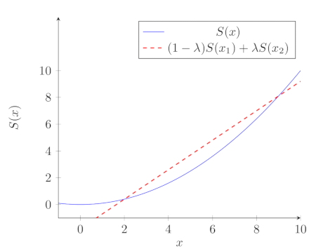
Let \(x_1 = 0\), then we have \( S(\lambda x_2) \leq \lambda S(x_2)\), for any \(x_2 \geq 0\) and any \( \lambda \in [0,1]\). Now consider \( \lambda_1 = \frac{x}{x+y}\) and \(x_2 = x + y\), then we have

$$ \begin{align} &S( \frac{x}{x+y}[x+y]) \\ &\leq \frac{x}{x+y} S(x+y) \\ \end{align} $$

which gives us

$$ \begin{align} &S(x) \leq \\ &\frac{x}{x+y}S(x + y) \tag{2}\label{2} \\ \end{align} $$

Similarly, if we set \(\lambda_2 = \frac{y}{x+y}\), we get

$$ \begin{align} &S(y) \leq \\ &\frac{y}{x+y} S(x+y) \tag{3}\label{3} \\ \end{align} $$

adding (2) to (3) we get

$$ \begin{align} &S(x) + S(y) \leq \\ &S(x + y) \tag{4}\label{4} \\ \end{align}

QED

Using that lemma, we see that since \(T(0) = 0\), all we have to do is suppose that \(T(n)\) grows at least as fast as \(cn\) (it could be much worse, like \(ce^{n}\)) to conclude that

$$ \begin{align} &T(\left\lceil { 0.2n} \right\rceil) + T( \left\lceil {0.71n} \right\rceil) \leq \\ &T( \left\lceil {0.2n}\right\rceil + \left\lceil {0.71n}\right\rceil) \\ \end{align} $$

It’s not hard to show that for large enough \(n\),

$$ \begin{align} &\left\lceil {0.2n}\right\rceil + \left\lceil {0.71n}\right\rceil \leq \\ &\left\lceil { 0.95n } \right\rceil \\ \end{align} $$

Putting this all together with equation (1) from above, we get

$$ \begin{align} &T(n) \leq \\ &c \left\lceil 0.2n \right\rceil + T(\left\lceil 0.95n \right\rceil) \tag{5}\label{5} \\ \end{align} $$ Using the “Almost the Master Theorem” from (More on Sorting and Analyzing Run Time Complexity), with equation (5) we can conclude that \(T(n) \in O(n) \). The proof that we gave, though, shows that \(T(n)\) “almost” didn’t make it. It was almost in \(O(n\log_2(n))\). Mathematically, that might not make a whole lot of sense, either a function is in \(O(n)\), or it isn’t, but in practice, it might take a while for \(T(n)\) to behave linearly.

We tested our program on 9000 randomly generated inputs with lengths that ranged from 10,000 elements to 100,000 elements. We counted the number of steps kth_smallest(input_array, k) took to separate input_array into the smallest k elements to the left, where k was chosen uniformly at random among all of the possible indices. Here’s a plot showing the distribution of the number of steps vs the length of the input array.

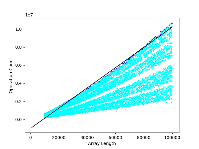
We’ve fit a line to the points that represent the most steps for a given input size. You can see that the actual upper limit seems to be convex. This means that for input sizes smaller than 100,000 elements, the run time isn’t behaving linear yet. That’s something that can happen in practice with real algorithms. Just because a function behaves linearly as it approaches infinity doesn’t mean it will do that in the range of real-world situations. We never get that close to infinity, afterall. On the other hand, testing only below 100,000 isn’t really testing for very large real-world applications. Real data can have trillions of entries.

We want to point out that this function can be added to quick_sort, which we will call “quick_sort_plus”, which we can show is in \(O(n\log_2(n))\). Here we’ve re-written quick_sort so that it uses the pivot() function implemented above.

quick_sort

 1
 2
 3
 4
 5
 6
 7
 8
 9
10
11
12
13
14
15

void quick_sort(int64_t* input, int64_t length)
{
  quick_sort(input, 0, length);
}
void quick_sort(int64_t* input, int64_t start, int64_t end)
{
  if(end - start < 2)
  {
    return;
  }
  int64_t k = pivot(&input[start], end - start) + start;
  
  quick_sort(input, start, k);
  quick_sort(input, k + 1, end);
}

quick_sort_plus

Here’s our implementation of quick_sort_plus(). Notice how similar the two are.

 1
 2
 3
 4
 5
 6
 7
 8
 9
10
11
12
13
14
15
16

void quick_sort_plus(int64_t* input, int64_t length)
{
  quick_sort_plus(input, 0, length);
}
void quick_sort_plus(int64_t* input, int64_t start, int64_t end)
{
  if(end - start < 2)
  {
    return;
  }
  int64_t m = (start + end) / 2;
  kth_smallest(&input[start], m - start, end - start);

  quick_sort_plus(input, start, m);
  quick_sort_plus(input, m + 1, end);
}

Since kth_smallest() runs in \(O(n)\) time, it is bounded by some \(cn\), for some \(c \in \mathbb{R}\). Thus \(T(n)\) for quick_sort_plus is less than or equal to \(cn + 2T(\left\lceil {\frac{n}{2}}\right\rceil) \), and that means that it is in \(O(n\log_2(n))\).

QED

Now we’re going to show that quick_sort can take \(O(n^2)\) steps to complete when given the worst input. The worst input is one which is in reverse order, so \( \text{input} = [a_0, a_1, … , a_{n-1}]\), where \( a_0 > a_1 > … > a_{n-1}\). When this is the case pivot takes \(n-1\) steps to send \(a_0\) to the rightmost position of the array (which is where it belongs, since it’s the largest element). In doing so, it doesn’t change the relation of any of the other elements with respect to each other. For example, if \( \text{input} = [5,4,3,2,1] \), then when pivot finishes, \( \text{input} = [4,3,2,1,5] \). \(5\) is now in the far right position, where it belongs, and everything else has been moved one position to the left. The index returned by pivot is \(n-1\), so when the two recursive calls to quick_sort are executed, one will have length \(n-1\) and the other will have length \(0\). Now the call to quick_sort that has input length \(n-1\) is in almost the exact same situation as the original call to quick_sort, except that its input is one element shorter. This is because its input is also in reverse order. Thus we will have to recursively sort sub-arrays of length \(n-1, n-2, n-3, … , 2, 1\), before we finish. For the recursive call with input of length \(m\), quick_sort calls the pivot subroutine, which will take \(cm\) steps to complete. Therefore, the entire execution of quick_sort on this input will take

\[ \sum\limits_{m = 1}^{n} cm = c\frac{n(n+1)}{2} \]

steps. Therefore quick_sort is in \(O(n^2)\).

QED

We want to point out, though, that in practice the original quick_sort is very good. We ran a similar test with quick_sort and quick_sort_plus to what we did above with kth_smallest. We counted the number of steps it took each to sort 9000 randomly generated arrays with lengths ranging from 10,000 elements to 100,000 elements. We tested both algorithms on the exact same set of randomly generated arrays. Here are the results for quick_sort:

Runtime Plots

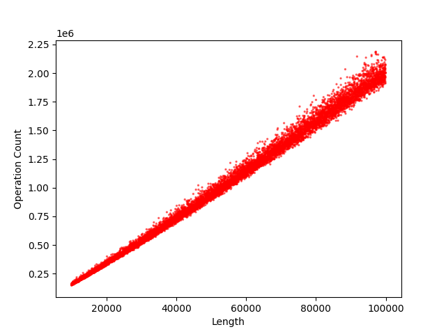
Here are the results for quick_sort_plus:

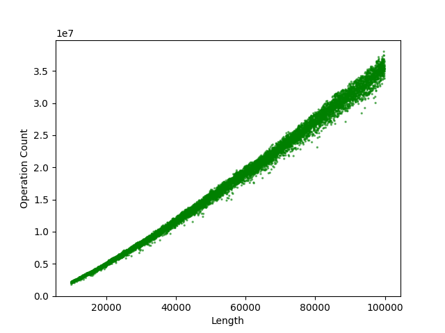
They may look similar enough, but the vertical scale isn’t the same. Here’s what we get when we merge the two into one scatter plot:

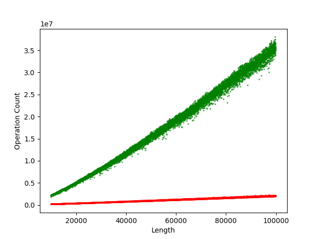
The results are kind of shocking. The plain quick_sort implementation greatly outperformed quick_sort_plus! The results aren’t even close. It turns out that the arrays that take ordinary quick_sort a long time to sort are incredibly rare. If you’re worried about one of those slowing your system down, you can simply check the value that pivot returns. If it’s too small or too large, so that the two sub-arrays are heavily imbalanced, simply randomly permute the array, and try again. Applying a random permutation can be done in \(O(n)\) steps. The chances that you’ll have to permute the array more than a couple times are extremely low.

That’s all for this entry!